
Yasmina Papadopoulos
FY2 Doctor, NHS Lothian, Scotland
The human visual system is often compared to a digital camera, with a lens focusing light onto a high-resolution sensor. This analogy is fundamentally flawed because it ignores the vast amount of processing done by the visual pathway. The retina and visual cortex do not passively record light; they continuously interpret it. When these processing rules are deliberately overloaded, we observe optical illusions. Here, I utilise eight optical illusions to illustrate different aspects of the workings of the visual system.
1. Troxler Fading illusion
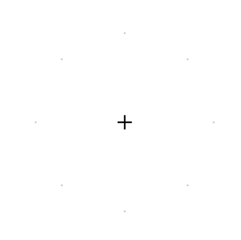
Fig. 1. The Troxler Fading illusion.
- How to interact: Stare at Fig. 1 at a normal reading distance. Fixate your gaze on the central black cross for 15 to 20 seconds, without shifting your gaze. Within seconds, the faint peripheral spots will begin to fade and may disappear completely, leaving a blank white page surrounding the cross.
- Ophthalmic explanation: Neurons in the visual pathway respond strongly to change and adapt to unchanging stimuli. Small involuntary eye movements normally refresh the image on the retina, but they are too small to move a faint, blurred-edged peripheral stimulus across a distinct boundary. Troxler fading is therefore attributed to neural adaptation, with contributions from both the retina and the visual cortex, rather than to exhaustion of photopigment. Because receptive fields are larger in the periphery, the effect is stronger there, and the unchanging stimulus drops out of conscious perception as the brain fills in the surrounding background.
- Where it comes from: It is named after Ignaz Paul Vital Troxler, a Swiss physician and philosopher, who described the effect in 1804 while studying how stationary objects in the periphery vanish from awareness when the gaze is held steady (1).
2. Opponent-Process afterimage illusion
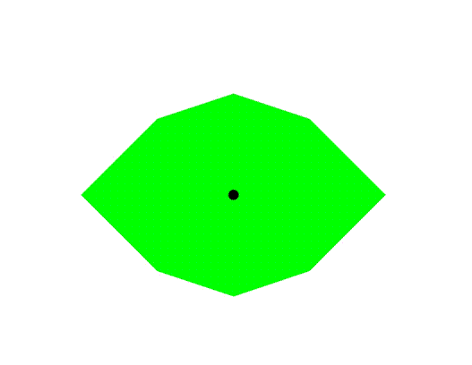
Fig. 2. The Opponent-Process afterimage illusion.
- How to interact: Stare at Fig. 2 at a normal reading distance. Fixate your gaze on the central black dot for 15 to 20 seconds. Then, immediately shift your gaze to a blank white sheet of paper, and a magenta eye-shaped profile will appear on the white surface.
- Ophthalmic explanation: This illustrates cone adaptation and chromatic opponency. Prolonged, steady fixation on a highly saturated green target adapts (bleaches) the middle-wavelength cones (M-cones) in a localised region of the retina. When the gaze shifts to a white surface, which reflects all visible wavelengths, the adapted M-cones respond weakly while the long-wavelength (L) and short-wavelength (S) cone signals are relatively unopposed. Because L and S cone signals together signal red plus blue, the visual system perceives magenta, the complementary colour to green. The afterimage fades as the cones recover.
- Where it comes from: The name stems from the opponent-process theory of colour vision, formulated by the German physiologist Ewald Hering in 1878 (2). Hering challenged the prevailing trichromatic theory, in which separate red-, green- and blue-sensitive receptors were thought to transmit their signals independently to the brain. He argued that colour is encoded in three opposing pairs: red versus green, blue versus yellow, and black versus white. Looking at red excites the first channel, while looking at green inhibits it. Because a single neural pathway cannot be excited and inhibited at the same time, we never see a greenish-red.
3. The Blind Spot Finder
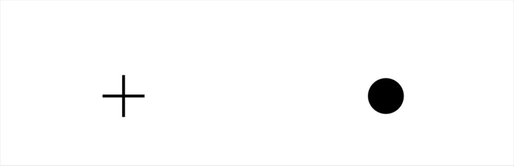
Fig. 3. The Blind Spot Finder.
- How to interact: Cover your left eye and stare at the cross in Fig. 3 with the right eye. Hold the page at arm’s length and slowly move it closer to your face. At some point, the black circle on the right will vanish, seamlessly replaced by the blank white background.
- Ophthalmic explanation: This experiment maps the location of the optic disc. As you alter the reading distance, you shift where the image of the black circle falls on the retina. At a specific distance, light from the circle lands on the blind spot, the region of the nasal retina that has no rods or cones, where the retinal ganglion cell axons bundle to exit the globe. The visual system receives no information from this location and fills in the gap using the surrounding white background.
- Where it comes from: The blind spot was described in 1660 by the French physicist Edme Mariotte, who published his account in 1668 (3). He is reported to have demonstrated it to the court of King Charles II of England by showing that a person’s head could vanish from view when its image fell on the blind spot.
4. The Scintillating Grid
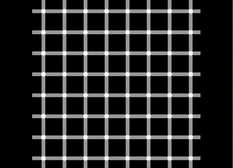
Fig. 4. The Scintillating Grid.
- How to interact: Scan your eyes casually back and forth across Fig. 4. Dark, ghostly spots will flash and dance inside the white discs at the intersections in your peripheral vision, but they vanish the moment you look directly at them.
- Ophthalmic explanation: The scintillating grid is a variant of the Hermann grid, in which dark spots appear at the intersections of a white grid on a black background (4). The classical explanation is lateral inhibition: a retinal ganglion cell in the periphery has a large receptive field and receives more inhibition at an intersection, where bright arms lie in four directions, than along a single arm, so the intersection appears darker. Cells at the centre of vision (the fovea) have receptive fields small enough to fit inside the white disc, so the illusion disappears under direct gaze. This account is now debated: later work indicates that orientation-selective cortical mechanisms contribute, and that simple centre-surround inhibition cannot explain every feature of the illusion (5,6).
- Where it comes from: The scintillating grid was described in 1994 by Elke and Bernd Lingelbach, who noticed the flashing effect in a modified Hermann grid, and was formally reported by Schrauf, Lingelbach and Wist in 1997 (5).
5. The Café Wall Illusion
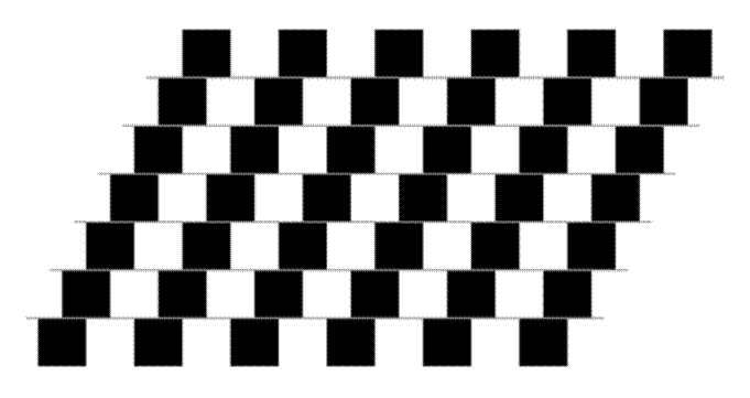
Fig. 5. The Café Wall Illusion.
- How to interact: Look at the grey lines in Fig. 5. Your brain will insist that the lines are tilted. When checked with a ruler, the lines are horizontal and parallel.
- Ophthalmic explanation: The distortion arises early in the visual pathway. Alternating, staggered black and white tiles produce local brightness changes at the grey mortar lines that early visual neurons interpret as slightly tilted edges. Models based on centre-surround retinal responses followed by orientation-selective cortical processing (V1) can reproduce the effect, and the misreading is then integrated across the row (7,8).
- Where it comes from: The pattern is named after the tiled wall of a café in Bristol, UK, where it was noticed in the 1970s by a member of Richard Gregory’s laboratory. Gregory and Heard published the first systematic study of the illusion in 1979 (Fig. 6) (7).

Fig 6. Professor Richard Gregory outside the café on St Michael’s Hill, Bristol, associated with the discovery of the Café Wall Illusion in the 1970s. Photograph by Steven Battle (2010). Source: Wikimedia Commons. Photo URL: https://commons.wikimedia.org/wiki/File:CafeWall.jpg. Licensed under Creative Commons Attribution-ShareAlike 3.0 (CC BY-SA 3.0): https://creativecommons.org/licenses/by-sa/3.0/

6. The Fraser Spiral
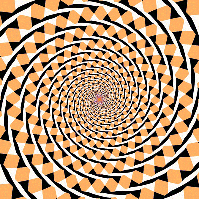
Fig. 7. The Fraser Spiral.
- How to interact: Scan your gaze casually across the whole of Fig. 7. The image gives the impression of an inward-winding spiral. When traced with a pen, however, your hand will follow a series of closed, concentric circles that never go inward.
- Ophthalmic explanation: The twisted-cord elements are consistently tilted relative to the true circular path. Orientation-selective neurons in the primary visual cortex (V1) register this local tilt, and later stages of visual processing integrate these local signals into a global spiral, overriding the true concentric layout (8,9).
- Where it comes from: It is named after James Fraser, a British psychologist who published a description of the pattern in 1908, which he called the “twisted cord” illusion (9).
7. The Kanizsa Star

Fig. 8. The Kanizsa Star.
- How to interact: Look at the centre of Fig. 8. The brain perceives a solid yellow star lying on top of the black circles, with edges that seem to extend across gaps where no line is drawn. Cover two of the black circles with your fingers and the sharp foreground star collapses into a flat, disjointed arrangement.
- Ophthalmic explanation: The brain treats the alignment of the black cut-outs and line breaks as too regular to be coincidence. It infers an occluding foreground object lying on top of the black circles. Neurons in visual cortical area V2 respond to these illusory contours as though a physical edge were present.10,11 Illusory contours of this type are often accompanied by a perceived brightness difference between the inside of the shape and its surround, although in an all-yellow figure like this one the effect is subtle.
- Where it comes from: It is named after Gaetano Kanizsa, an Italian psychologist who first published the illusory-triangle figure in 1955 (10). Kanizsa was also a painter, and his interest in how artists create forms from minimal cues helped shape his research. The neural basis of illusory contours was later shown in V2 by von der Heydt, Peterhans and Baumgartner in 1984 (11).
8. The Ebbinghaus Illusion
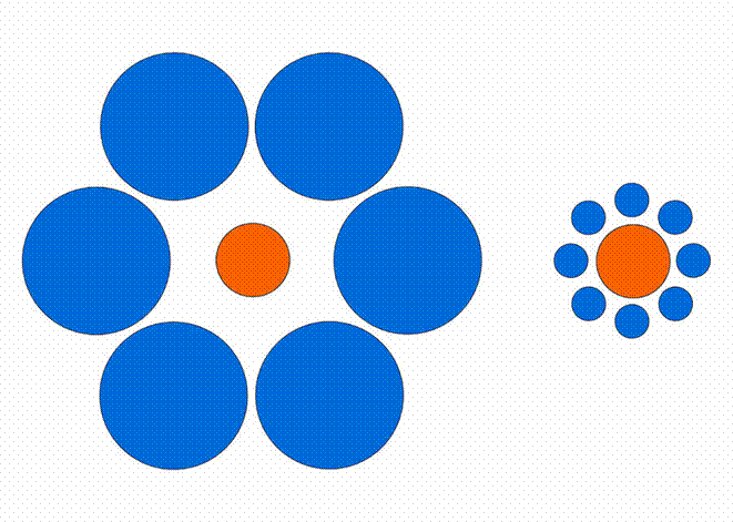
Fig. 9. The Ebbinghaus Illusion.
- How to interact: Look at both orange circles in Fig. 9 and compare their sizes. The orange circle surrounded by small blue circles looks larger, while the one surrounded by large blue circles looks smaller, although both are identical.
- Ophthalmic explanation: Perceived size depends on context. The visual system judges the size of an object relative to its neighbours rather than in isolation. Functional imaging shows that the strength of the illusion in individuals correlates with the surface area of their primary visual cortex (V1), indicating that early cortical processing contributes alongside higher-level mechanisms (12).
- Where it comes from: The illusion is named after Hermann Ebbinghaus, the German psychologist best known for his pioneering work on memory, and it appears in his 1897 textbook. It was popularised in English-language psychology by Edward Titchener in 1901, and is therefore also known as the Titchener circles illusion (13).
Conclusions
These optical illusions illustrate how the visual pathway is a complex processor that prioritises edge detection, contrast and context over literal physical properties.
- Optical illusions 1–4 probe mechanisms that begin at the level of the retina. They demonstrate neural adaptation (1), cone adaptation and colour opponency (2), the anatomical blind spot (3), and lateral inhibition, although the neural basis of the scintillating grid remains debated (4). Troxler fading also has a cortical component.
- Optical illusions 5 and 7 show how orientation-selective neurons in the early visual cortex (V1) mistake local edges, angles and contrast borders for tilted lines. In the Fraser spiral, later stages of processing then group these local errors into a false global spiral.
- Optical illusions 8 and 9 show the role of context and inference. In the Kanizsa star, V2 neurons respond to illusory contours and the brain would rather perceive an imaginary foreground star than accept disjointed fragments. In the Ebbinghaus illusion, the perceived size of an object is set by its surroundings, with the involvement of V1.
The same constructive machinery that hides our blind spot from us also explains why advanced sight loss may cause people to see vivid things that are not there, such as faces, figures, animals, patterns and landscapes, and sometimes very small people (Charles Bonnet syndrome). Ultimately, what we ‘see’ is not a direct print of the world, but a computationally distorted mental model that attempts to make sense of the image.
References
- Troxler IPV. Über das Verschwinden gegebener Gegenstände innerhalb unseres Gesichtskreises. In: Himly K, Schmidt JA, eds. Ophthalmologische Bibliothek. Vol 2, part 2. Jena: Fromann; 1804:1–53.
- Hering E. Zur Lehre vom Lichtsinne. Vienna: Carl Gerold’s Sohn; 1878.
- Mariotte E. A new discovery touching vision. Philos Trans R Soc Lond. 1668;3:668–669.
- Hermann L. Eine Erscheinung simultanen Contrastes. Pflügers Arch Gesamte Physiol. 1870;3:13–15.
- Schrauf M, Lingelbach B, Wist ER. The scintillating grid illusion. Vision Res. 1997;37(8):1033–1038.
- Schiller PH, Carvey CE. The Hermann grid illusion revisited. Perception. 2005;34(11):1375–1397.
- Gregory RL, Heard P. Border locking and the Café Wall illusion. Perception. 1979;8(4):365–380.
- Morgan MJ, Moulden B. The Münsterberg figure and twisted cords. Vision Res. 1986;26(11):1793–1800.
- Fraser J. A new visual illusion of direction. Br J Psychol. 1908;2(3):307–320.
- Kanizsa G. Margini quasi-percettivi in campi con stimolazione omogenea. Riv Psicol. 1955;49(1):7–30.
- von der Heydt R, Peterhans E, Baumgartner G. Illusory contours and cortical neuron responses. Science. 1984;224(4654):1260–1262.
- Schwarzkopf DS, Song C, Rees G. The surface area of human V1 predicts the subjective experience of object size. Nat Neurosci. 2011;14(1):28–30.
- Titchener EB. Experimental Psychology: A Manual of Laboratory Practice. Vol 1. New York: Macmillan; 1901.